De la qualité de l’air

Capteur de CO₂ Aranet4 vu de faceLa pandémie de COVID-19 a mis en lumière de nombreux éléments de notre quotidien auxquels nous n'étions pas habitués à prêter attention : l'impact des différents gestes "barrière" sur la transmission, mais aussi le traitement que l'on applique (ou pas) à notre air intérieur.
En raison de l'activité humaine, la quantité de CO₂ dans l'air dans une concentration urbaine de bonne taille se situe autour de 400 à 450 ppm. En milieu clos la concentration mesurée va dépendre de l'activité, du nombre de personnes et de la qualité de l'aération. Si on exclut les cas où le CO₂ est produit par les plantes et des activités artificielles (gazinière par exemple) alors le CO₂ que vous mesurez dans une pièce peut être corrélé à la quantité d'air sortant des poumons des mammifères présents et passés dans la pièce.
Pour faire simple, une valeur haute montre un déficit d'aération et donc votre risque de contamination peut augmenter et vos capacités cognitives baissent.
"Pour la science" et parce que je suis un irrécupérable geek, j'ai décidé de tester trois capteurs permettant la mesure en continu du taux de CO₂ dans l'air ambiant. J'ai choisi trois appareils tout-faits donc utilisables par le grand public presque sans aucune connaissance technique.

Caractéristiques générales

Aranet4 Home Mini Carbon Dioxide Monitor SCD4x CO₂ Gadget
affichage écran e-ink écran à crystaux liquides 1 LED
historique 7 jours sans 8192 mesures
interface utilisateur app iOS et Android bouton unique app iOS et Android
données CO2, température, humidité, pression atmosphérique CO2 CO2
alerte son et visuel son et visuel visuel (LED rouge)
accès distant Bluetooth sans Bluetooth
source d'energie 2 piles AA batterie interne port USB
autonomie quelques mois à plusieurs années 7 heures sans
prix 261,60 € 64,90 € 71,92 €

(les prix s'entendent TTC et frais de port inclus)

Bilan des expérimentations

J'ai utilisé ces capteurs en conditions réelles : maison, travail, transport, cinéma, etc. Ils utilisent tous trois la technologie NDIR (non-dispersive infra-red) aussi je m'attendais à ce qu'ils fournissent tous des mesures similaires. Ce n'est pas le cas, mais finalement ce n'est pas forcément ce qui retient l'attention à la fin de la journée.

Mesures

Sur la qualité des mesures, les capteurs Aranet4 Home et SCD4x CO₂ Gadget (Sensirion) sont ceux qui donnent les meilleurs résultats : ils sont très proches l'un de l'autre avec un écart qui dépasse très rarement les 50 ppm. En comparaison le Mini Carbon Dioxide Monitor (MCDM) sous-évalue la concentration de CO₂ de 160 à 200 ppm.
Le gagnant de cette catégorie est le modèle Aranet4 qui propose en plus du CO₂ une mesure de la température, de l'humidité et de la pression.

Ergonomie

Capteur de CO₂ avec son mousqueton
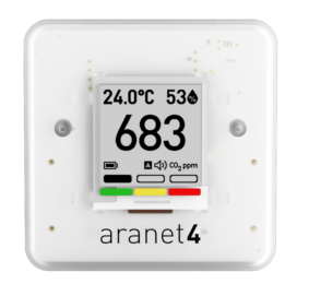
L'ergonomie se mesure à l'aune des usages de chacun. J'attache pour ma part une grande importance à la qualité des interactions avec les appareils et je n'aime pas la friction dans l'usage quotidien. Pour moi, c'est à nouveau l'Aranet4 qui remporte la palme avec son écran e-ink qui reste lisible tout le temps sans drainer les piles. Une fois paramétré via une application smartphone assez bien faite, plus besoin d'y revenir. C'est agréable.
Il tient aussi tout seul quand on le pose, ce qui n'est pas le cas du MCDM. Ce dernier n'est pas conçu pour être posé à la verticale. On peut le coucher mais cela bloque une partie de la circulation de l'air dans le capteur. L'ergonomie du MCDM est d'ailleurs une catastrophe avec un unique bouton pour tout faire : allumer, éteindre, sortir de veille, calibrer, activer ou désactiver les alertes sonores. Son maniement est pénible et déstabilise certains utilisateurs. Pour les fans de mobilité par contre, le MCDM est sans doute plus ergonomique puisque qu'il est conçu pour être accroché à la ceinture, à un sac, via un mousqueton métallique lourd et robuste.

Autonomie

Bien que clairement conçu pour la mobilité le MCDM pêche par une autonomie catastrophique, tout juste 7 heures. Si vous l'emmenez au travail le matin, il sera vide avant la fin de votre journée et devra être rechargé (câble USB-A vers USB-C fourni). En cause une batterie de taille modeste, le rafraîchissement très rapide des mesures et un écran LCD.
Le modèle Aranet4 dispose quant à lui d'une autonomie record avec juste 2 piles AA. L'écran e-ink y est pour beaucoup mais il ne faut pas oublier que la transmission des données se fait en Bluetooth ce qui est aussi consommateur. L'Aranet4 permet par contre de régler la fréquence de rafraîchissement des mesures ce qui a un effet important sur l'autonomie.
Le SCD4x CO₂ Gadget n'a pas de source d'énergie propre, il doit être branché sur un port USB-A pour être alimenté.
La palme revient évidemment à l'Aranet4 une fois de plus.

SCD4x CO₂ Gadget de sensirion avec sa boîte verte

Gestion des données

L'Aranet4 et le SCD4x CO₂ Gadget peuvent tous les deux stocker des données de mesure pendant un certain temps. L'Aranet4 annonce une rétention de 7 jours, le SCD4x CO₂ Gadget annonce un nombre de points de mesure (l'intervalle de temps entre deux mesures est réglable dans l'application). Les deux disposent d'une application de smartphone pour récupérer les données de l'historique. L'une comme l'autre permettent d'exporter les données, ce qui est sympa si vous souhaitez conserver un historique sur le long terme. Attention cependant, si le SCD4x CO₂ Gadget n'est plus alimenté il oubliera les données enregistrées. L'Aranet4 obtient à nouveau la première place, talonné de près par le SCD4x CO₂ Gadget, largement devant le MCDM qui ne gère aucun historique des mesures.

App et divers

L'Aranet4 et le SCD4x CO₂ Gadget sont tous les deux dépendants d'une application plutôt bien faite dans les deux cas. Ces applications permettent différents réglages sur les appareils ainsi que l'affichage et l'export des données enregistrées sur les appareils. L'Aranet4 et son application sont aussi sécurisés : il faut en effet explicitement apparier la sonde avec l'application au moyen d'un code (manipulation classique avec les appareils bluetooth). L'application permet en plus de mettre à jour le firmware de la sonde. Côté SCD4x par contre, pas de manipulation d'appariement. C'est un peu moyen en termes de sécurité. L'application vérifie aussi la version du firmware de la sonde mais je ne sais pas si elle propose un mécanisme pour pousser une mise à jour le cas échéant.

Podium

Pour moi, la première place revient à l'Aranet4 qui, en dépit d'un prix très élevé, apporte une véritable solution clé en main, complète, fiable et, autant que je puisse en juger, durable.
La seconde place revient au SCD4x CO₂ Gadget. Il est d'une grande simplicité, il est petit et performant ce qui le rend attractif malgré sa dépendance à une source de courant extérieure. Son application est bien faite et j'aime le sens du détail avec le quel tout est pensé (on peut régler l'intensité de la LED).
Bon dernier le Mini Carbon Dioxide Monitor, avec une batterie fixe dont l'autonomie est en contradiction totale avec son ambition de mobilité et qui a un impact très négatif sur la durée de vie probable du produit. Une qualité de mesure légèrement inférieure aux deux autres et une ergonomie affreuse viennent encore noircir le tableau. Mais c'est aussi un modèle très abordable compte tenu du fait qu'il utilise la technologie NDIR.
Je pense qu'il est important de souligner que bon nombre de capteurs de CO₂ vendus sur des sites comme Amazon sont basés sur des technologies très inférieures en termes de qualité et de performance. Certains sont aussi vendus avec la mention NDIR alors qu'ils n'utilisent pas cette technologie. Les trois capteurs que j'ai testés sont parmi les meilleurs dans l'offre grand public.

Si l'argent n'est pas un problème ou si vous avez absolument besoin d'un capteur autonome, lisible par tous, à poser dans un coin et à oublier, achetez un Aranet4.
Si vous voulez seulement un point de mesure fixe sans trop dépenser et que lire les mesures sur une app vous convient, achetez le SCD4x CO₂ Gadget de Sensirion.
Si vous avez besoin, quelques heures dans la journée, d'un capteur qui vous accompagne et qui soit capable de vous alerter très rapidement en cas de dépassement du seuil de CO₂ alors le format "accrochable" et la fréquence élevée de rafraîchissement du Mini Carbon Dioxide Monitor en font l'outil idéal.

photo du gadget de Sensirion branché sur un hub USB et de l'interface d'accueil de l'application de pilotage MyAmbience

SCD4x CO₂ Gadget branché sur un hub USB, écran d'un système sous macOS faisant tourner l'app iOS MyAmbience de Sensirion

Related posts

Cracking passwords: testing PCFG password guess generator

Cracking passwords is a kind of e-sport, really. There's competition among amateurs and professionals "players", tools, gear. There are secrets, home-made recipes, software helpers, etc.
One of this software is PCFG password guess generator, for "Probabilistic Context-Free Grammar". I won't explain the concept of PCFG, some scientific literature exists you can read to discover all the math inside.
PCFG password guess generator comes as two main python programs: pcfg_trainer.py and pcfg_manager.py. Basic mechanism is the following:
- you feed pcfg_trainer.py with enough known passwords to generate comprehensive rules describing the grammar of known passwords, and supposedly unknown passwords too.
- you run pcfg_manager.py, using previously created grammar, to create millions of password candidates to feed into your favorite password cracker (John the Ripper, Hashcat…).

In order to measure PCFG password guess generator's efficiency I've made few tests. Here is my setup:

  • Huge password dump, 117205873 accounts with 61829207 unique Raw-SHA1 hashes;
  • John the Ripper, Bleeding Jumbo, downloaded 20160728, compiled on FreeBSD 10.x;
  • PCFG password guess generator, downloaded 20160801, launched with Python 3.x;

Here's my methodology:

Of these 61829207 hashes, about 35 millions are already cracked. I've extracted a random sample of 2 millions known passwords to feed the trainer. Then I've used pcfg_manager.py to create a 10 millions lines word list. I've also trimmed the famous Rockyou list to it's 10 millions first lines, to provide a known reference.

Finally, I've launched this shell script:

#!/bin/sh
for i in none wordlist jumbo; do
  ./john --wordlist=pcfg_crckr --rules=$i --session=pcfg_cracker-$i --pot=pcfg_cracker-$i.pot HugeDump
  ./john --wordlist=ry10m --rules=$i --session=ry10m-$i --pot=ry10m-$i.pot HugeDump
done

No forking, I'm running on one CPU core here. Each word list is tested three times, with no word mangling rules, with defaults JtR rules, and finally with Jumbo mangling rules.

Some results (number of cracked passwords):

Rules PCFG Rockyou
none 4409362 2774971
wordlist 5705502 5005889
Jumbo 21146209 22781889

That I can translate into efficiency, where efficiency is Cracked/WordlistLength as percentage:

Rules PCFG Rockyou
none 44.1% 27.7%
wordlist 57.1% 50.1%
Jumbo 211.5% 227.8%

It's quite interesting to see that the PCFG generated word list has a very good efficiency, compared to Rockyou list, when no rules are involved. That's to be expected, as PCFG password guess generator has been trained with a quite large sample of known passwords from the same dump I am attacking.
Also, the PCFG password guess generator creates candidates that are not very well suited for mangling, and only the jumbo set of rules achieves good results with this source. Rockyou on the other hand starts quite low with only 27.7% but jumps to 50.1% with common rules, and finally defeats PCFG when used with jumbo rules.

On the word list side, Rockyou is known and limited: it will never grow. But PCFG password guess generator looks like it can create an infinite list of candidates. Let see what happens when I create a list of +110 M candidates and feed them to JtR.

Rules PCFG Efficiency
none 9703571 8.8%
wordlist 10815243 9.8%

Efficiency plummets: only 9.7 M hashes cracked with a list of 110398024 candidates, and only 1.1 M more when the set of rules "wordlist" is applied. It's even less beneficial than with a list of 10 M candidates (+1.3 M with "wordlist" rules, compared to "none").

On the result side, both word list with jumbo rules yields to +21 M cracked passwords. But are those passwords identical, or different?

Rules Total unique cracked Yield
none 6013896 83.7%
wordlist 8184166 76.4%
Jumbo 26841735 61.1%
Yield = UniqueCracked / (PcfgCracked + RockyouCracked)

A high yield basically says that you should run both word lists into John. A yield of 50% means that all pwd cracked thanks to PCFG are identical to those cracked with the Rockyou list.

As a conclusion, I would say that the PCFG password guess generator is a very interesting tool, as it provides a way to generate valid candidates pretty easily. You probably still need a proper known passwords corpus to train it.
It's also very efficient with no rules at all, compared to the Rockyou list. That might make it a good tool for very slow hashes when you can't afford to try thousands of mangling rules on each candidate.

Some graphs to illustrate this post:

every john session on the same graph

every john session on the same graph

every session, zoomed on the first 2 minutes

every session, zoomed on the first 2 minutes

Rules "wordlist" on both lists of candidates

Rules "wordlist" on both lists of candidates

Rules "none", both lists of candidates

Rules "none", both lists of candidates

Related posts

ZFS primary cache is good

Last year I've written a post about ZFS primarycache setting, showing how it's not a good idea to mess with it. Here is a new example based on real world application.
Recently, my server crashed, and at launch-time Splunk decided it was a good idea to re-index a huge apache log file. Apart from exploding my daily index quota, this misbehavior filed the index with duplicated data. Getting rid of 1284408 events in Splunk can be a little bit resource-intensive. I won't detail the Splunk part of the operation: I've ended up having 1285 batches of delete commands that I've launched with a simple for/do/done bash loop. After a while, I noticed that the process was slow and was making lots of disk IOs. Annoying. So I checked:

# zfs get primarycache zdata/splunk
NAME          PROPERTY      VALUE         SOURCE
zdata/splunk  primarycache  metadata      local

Uncool. This setting was set locally so that my toy (Splunk) would not harvest all ARC from the server, hurting production. For efficiency's sake, I've switched back the primary cache to all:

# zfs set primarycache=all zdata/splunk

Effect was almost instantaneous: ARC filled with Splunk data and disk IOs plummeted.

primarycache # of deletes per second
metadata 10.06
all 22.08

A x2.2 speedup on a very long operation (~20 hours here) is a very good argument in favor of primarycache=all for any ZFS user.

acceleration of a repetitive splunk operation thanks to ZFS primarycache setting

Acceleration of a repetitive splunk operation thanks to ZFS primarycache setting

Related posts

L4D2: comparative benchmark between Mac OS X and Windows

Back in december 2012 I've benchmarked (shortly) native and virtualized Mac OS X against virtualized Windows.
Few days ago, I've dedicated a 250G B SSD to a Windows 7 installation, inside my Mac Pro. Weird thing for me to go back and forth between Mac OS X and Windows. I'm more accustomed to +50 days long uptime. Admittedly my various attempts to put Mac OS X into deep sleep, reboot on Windows, and go back later to a fully restored Mac OS X session right out from deep sleep, are failing. That's another story.
Nevertheless, I'm using this Windows system as a playground.

Inside this Mac Pro model 2010, I've one Xeon quad core 2.8 GHz with 24 GB RAM, and a Radeon HD 5770. One SSD is dedicated to Mac OS X 10.6.8, and one SSD is dedicated to Windows 7 Pro 64 bits (with latest stable Catalyst drivers). Both systems are using the latest Steam client with a fully updated and clean Left 4 Dead 2 install.

I've recorded a demo, and played back this file on both systems with identical video settings, recording fps numbers during the playback. The demo is 17827 frames long, and video settings are "MSAA x4", "Anisotropic 8x", "vertical sync triple", "resolution 1920x1200", "shader detail very high', "effect detail high", "model/texture detail high".

The playback is a bit laggy on Mac OS X, especially when the player is looking at fire. It would be playable, but not a very smooth experience. The playback is better on Windows.
Here is the plot of numbers of frames calculated at a given fps rate. For example, on Mac OS X (black line) a total of 4 frames were calculated at a frame rate of 10 fps. On Windows, 90 frames where calculated at a frame rate of 47 fps.

click plot to display full size

click plot to display full size

Windows 7 has better drivers, and may be the game itself is coded better. The fact is some situations in the game are not handled very well by the GPU on Mac OS X. The huge spike around 30 fps means that ~2500 frames were computed at about 30 fps. Not good. But more importantly the global shape of the plot shows a spread of fps values from as low as 10 fps to 60 fps. Note that the log scale on Y does mask isolated frames (Y=1).
Windows does a better job here, with only a handful of frames below 40 fps.

Fortunately L4D2 is an old game, and my hardware is enough to handle it nicely even on Mac OS X (I usually play at 1600x1000), but being able to push it a little further with full quality on Windows is a nice thing. I hope L4D3 will run ok too, some day, in a not too distant future.

Edit

To complete the comparison, I've made a Cinebench R15 benchmark. The OpenGL score on Windows 7 is ~64 fps, and the same test on Mac OS X 10.6.8 is ~53 fps. On CPU side both OSes score around 440.

Related posts

ZFS primarycache: all versus metadata

In my previous post, I wrote about tuning a ZFS storage for MySQL. For InnoDB storage engine, I've tuned the primarycache property so that only metadata would get cached by ZFS. It makes sense for this particular use, but in most cases you'll want to keep the default primarycache setting (all).
Here is a real world example showing how a non-MySQL workload is affected by this setting.

On a virtual server, 2 vCPU, 8 GB RAM, running FreeBSD 9.1-RELEASE-p7, I have a huge zpool of about 4 TB. It uses gzip compression, and stores 1.8TB of emails (compressratio 1.61x) and 1TB documents (compressratio 1.15x). Documents and emails have their own dataset, on the same zpool.
As it's a secondary backup server, isolated from production, I can easily make some tests.

I've launched clamscan (the binary part of ClamAV virus scanner) against a small branch of the email storage tree (about 1/1000 of total emails) and measured the zpool IOs, CPU usage and total runtime of the scan.
Before each run, I've rebooted the server to clear cache.
clamscan is set up so that every temporary files are written into a UFS2 filesystem (/tmp).

One run was made with property primarycache set to all, the other run was made with primarycache set to metadata.

Total runtime with default settings primarycache=all is less than 15 minutes, for 20518 files:

Scanned directories: 1
Scanned files: 20518
Infected files: 2
Data scanned: 7229.92 MB
Data read: 2664.59 MB (ratio 2.71:1)
Time: 892.431 sec (14 m 52 s)

Total runtime with default settings primarycache=metadata is more than 33 minutes:

Scanned directories: 1
Scanned files: 20518
Infected files: 2
Data scanned: 7229.92 MB
Data read: 2664.59 MB (ratio 2.71:1)
Time: 2029.921 sec (33 m 49 s)

zpool iostat every 5 seconds, with different primarycache settings, ~10 minutes range.

zpool IO stats

CPU usage for clamscan process, and for kernel{zio_read_intr_0} kernel thread. 5 seconds sampling, with different primarycache settings, ~10 minutes range.

CPU stats

In both tests, the server is freshly rebooted, cache is empty. Nevertheless, when primarycache=all the kernel{zio_read_intr_0} thread consumes very few CPU cycles, and the clamscan process run's more than twice as fast as the same process with primarycache=metadata.
More importantly, clamscan manages to read the exact same amount of data in both tests, using 10 times less IO throughput when primarycache is set to all.

There is something weird. Let's make another test:

I create 2 brand new datasets, both with primarycache=none and compression=lz4, and I copy in each one a 4.8GB file (2.05x compressratio). Then I set primarycache=all on the first one, and primarycache=metadata on the second one.
I cat the first file into /dev/null with zpool iostat running in another terminal. And finally, I cat the second file the same way.

The sum of read bandwidth column is (almost) exactly the physical size of the file on the disk (du output) for the dataset with primarycache=all: 2.44GB.
For the other dataset, with primarycache=metadata, the sum of the read bandwidth column is ...wait for it... 77.95GB.

There is some sort of voodoo under the hood that I can't explain. Feel free to comment if you have any idea on the subject.

A FreeBSD user has posted an interesting explanation to this puzzling behavior in FreeBSD forums:

clamscan reads a file, gets 4k (pagesize?) of data and processes it, then it reads the next 4k, etc.

ZFS, however, cannot read just 4k. It reads 128k (recordsize) by default. Since there is no cache (you've turned it off) the rest of the data is thrown away.

128k / 4k = 32
32 x 2.44GB = 78.08GB

Damnit.

Related posts

Benchmark: virtualized OS X vs Windows

Lately I've discussed the performance drop between a virtualized Mac OS X and the same system running natively on a Mac Pro. My virtualization project is not limited to Mac OS X of course. Windows, Linux, FreeBSD are also part of the deal. In order to further test my virtualized workstation setup, I've created a Windows Server 2008 R2 VM.
Every VM runs on top of ESXi, only one VM at a time so no interference is possible. Each VM uses the ATI Radeon HD 5770 PCIe card directly thanks to VMware passthrough mode. ESXi is running on a Mac Pro, and the native OS X system runs on the same Mac Pro so I have a consistent hardware platform.

I've given Cinebench a ride on this Windows VM, and I must admit, results are appalling… for Mac OS X:

Cinebench OS X 10.8.2 native OS X 10.8.2 VM Windows Server 2008 R2 VM
CORES 4 4 4
LOGICALCORES 2 1 1
MHZ 2800 2663 2800
CBCPUX 5.038354 3.797552 3.962436
CBOPENGL 32.284100 27.319487 53.606468

I'm afraid a virtualized Windows system achieves better results than a native OS X. And not just a little bit better, but 66% better. We knew for ages that Apple ships crappy graphics card drivers and almost obsolete OpenGL. This is one more evidence.

After further research, I've finally succeeded in launching some Valve games on this windows VM: Half Life Lost Coast and Portal. They both run quite nicely. The HL Lost Coast integrated benchmark scores a very nice 229,82 FPS and the portal frame rate displayed by the command cl_showfps 1 was around 200 and 300.
On Team Fortress 2 I've been able to make a proper benchmark. That's not as detailed as my L4D2 bench, but that's enough.
I've recorded a game on TF2, Mac OS X 10.6.8, played it back with the timedemo command on the same system, and on the Windows VM.
It's a short demo (4099 frames) featuring a control point map with 12 players (11 bots, and me). Video settings were the same on both sides, of course.

Mac OS X 10.6.8 Native Windows VM
average 59.04 fps 59.83 fps
variability 2.764 fps 3.270 fps

It looks like something is capping the fps at 60. I don't know if it comes from my settings, or if it comes from outside the game. Both scores are very similar. Mac OS X's only bonus is the smaller variability, meaning its frame rate is more consistent throughout the demo. If only I had sound in my VMs…

Next step: try to configure a Ubuntu VM so it can use the ATI Radeon HD 5770 PCIe card, and make good use of my Steam On Linux beta test account.

Related posts

Mac OS X Benchmark: native vs virtualized, part 2

I've been really disappointed by my last benchmark of a virtualized Mac OS X running on top of ESXi with graphics card accessed in passthrough mode. So disappointed in fact that I had to make new tests.
This time, I've decided to ditch the six years old XBench, and to use proper video benchmarking tools: Geeks3D GpuTest, and Cinebench. And guess what? Thats better.
To run those tests, I've had to install OS X 10.8.2 because Geeks3D GpuTest doesn't run on Mac OS X 10.6.8. So I dedicated a SATA HDD on my Mac Pro to a fresh install of 10.8.2, created a VM with it and ran both benchmarks, once from the Mac Pro booted from OS X, once from the OS X VM.

In the chart bellow you can find FurMark and GiMark tests results for a native OS X system running on the Mac Pro, and for the exact same system running as a VM on top of ESXi hypervisor. No tuning was done, I've used the default settings for every benchmarks.

Geeks3D GpuTest Native VM
FurMark (AvgFPS / Score) 47 / 2845 47 / 2872
GiMark (AvgFPS / Score) 33 / 2000 7 / 446

FurMark scores the same frame rate on VM and on native OS X. But GiMark is not good at all, with a VM score 4.5x lower than reference.

Cinebench's results are quite interesting too:

Cinebench Native VM
CORES 4 4
LOGICALCORES 2 1
MHZ 2800 2663
CBCPUX 5.038354 3.797552
CBOPENGL 32.284100 27.319487

VM results are quite close from reference, but the CPU frequency is reported as 2.663 GHz instead of 2.8 GHz, and the VM has only 4 CPU threads, instead of 8. This explain the CPU performance drop between native and virtualized OS X. The OpenGL score is quite good, showing only a 15.4% drop.
We are very far from the 87% drop on XBench's OpenGL test.

On the left side the native OS X, on the right side the virtualized OS X:
Cinebench results for OS X 10.8.2 native vs virtualized

Related posts

Mac OS X Benchmark: native vs virtualized

An important thing about my work-in-progress virtualized workstation setup is that I've created the Mac OS X VM using my very own hard drives, hooked as raw devices (RDM: raw device mapping). So I can boot exactly the same OS directly from the hard drive, or from ESXi into a virtual machine. Quite convenient when the time comes to make comparisons. And now, I can boot the VM with ATI Radeon graphics card plugged in passthrough mode thanks to VMware DirectPath I/O and some tweaking.
While it's not enough to make a workstation (still miss a keyboard/mouse in passthrough), it allows some benchmarks. I've ran XBench on the VM and on the same OS booted natively from the hard drive.

The VM is configured with only 4 CPU. the Mac Pro sports a quad core Xeon capable of hyperthreading, so when Mac OS X boots natively it sees 8 CPU. It might explain the 50% difference on the Thread test, but that will require further testing.

The final result is not good at all. I understand very well that virtualization has a performance cost, but if I want a powerful virtualized workstation I need a setup that will waste as few resources as possible.
Quartz Graphics and User Interface tests show that "desktop" graphics are well supported, but the OpenGL test results are horrendous. With a performance loss of 87%, it predicts much trouble with games. According to this very simple benchmark, the VMware passthrough mode for graphics card seems to be very bad compared to what can be seen on XEN for example.
To be honest, having my hard disks accessed directly via RDM, I though I would have a 10-15% penalty. The 46% drop for sequential access surprises me. As for the GPU, the OpenGL results are so bad I'm wondering if the graphics card is properly passed through. May be some features are just dropped in the process. By the way, the virtualized Mac OS X won't load the screen color profile. May be it's related to the pseudo-VGA screen attached to the VSphere console. Unfortunately I can't get rid of this pseudo-VGA screen yet. Until I find a way to pass keyboard and mouse through to the VM, I need the VSphere console.

Results 259,39 127,18 -50,97 %
System Info
Xbench Version 1,3 1,3
System Version 10,6,8 (10K549) 10,6,8 (10K549)
Physical RAM 24576 MB 12288 MB
Model MacPro5,1 VMware7,1
Drive Type WDC WD1001FALS WDC WD1001FALS (ATA)
CPU Test 205,42 200,27 -2,51 %
GCD Loop 314,75 16,59 Mops/s 305,66 16,11 Mops/s -2,89 %
Floating Point Basic 182,81 4,34 Gflop/s 177,44 4,22 Gflop/s -2,94 %
vecLib FFT 121,5 4,01 Gflop/s 119,14 3,93 Gflop/s -1,94 %
Floating Point Library 385,38 67,11 Mops/s 374,17 65,15 Mops/s -2,91 %
Thread Test 954,74 477,33 -50,00 %
Computation, 4 thr. 989,65 20,05 Mops/s 517,69 10,49 Mops/s -47,69 %
Lock Contention, 4 thr. 922,22 39,67 Mlocks/s 442,8 19,05 Mlocks/s -51,99 %
Memory Test 452,72 370,19 -18,23 %
System 493,4 452,74 -8,24 %
Allocate 746,78 2,74 Malloc/s 877,63 3,22 Malloc/s 17,52 %
Fill 352,03 17116,62 MB/s 287,47 13977,29 MB/s -18,34 %
Copy 526,18 10867,96 MB/s 497,95 10285,00 MB/s -5,37 %
Stream 418,24 313,1 -25,14 %
Copy 422,51 8726,77 MB/s 321,23 6634,92 MB/s -23,97 %
Scale 395,84 8178,02 MB/s 303,88 6278,02 MB/s -23,23 %
Add 438,89 9349,24 MB/s 328,71 7002,18 MB/s -25,10 %
Triad 417,99 8941,89 MB/s 300,37 6425,59 MB/s -28,14 %
Quartz Graphics Test 315,19 300,47 -4,67 %
Line [50% α] 239,24 15,93 Klines/s 232,29 15,47 Klines/s -2,91 %
Rectangle [50% α] 314,61 93,93 Krects/s 296,25 88,45 Krects/s -5,84 %
Circle [50% α] 264,41 21,55 Kcircles/s 251,89 20,53 Kcircles/s -4,74 %
Bezier [50% α] 279,29 7,04 Kbeziers/s 263,55 6,65 Kbeziers/s -5,64 %
Text 875,44 54,76 Kchars/s 836,28 52,31 Kchars/s -4,47 %
OpenGL Graphics Test 306,01 39,01 -87,25 %
Spinning Squares 306,01 388,19 frames/s 39,01 49,49 frames/s -87,25 %
User Interface Test 463,72 405,19 -12,62 %
Elements 463,72 2,13 Krefresh/s 405,19 1,86 Krefresh/s -12,62 %
Disk Test 97,42 72,35 -25,73 %
Sequential 176,21 94,27 -46,50 %
Uncached Write [4K blk.] 180,38 110,75 MB/s 167,14 102,62 MB/s -7,34 %
Uncached Write [256K blk.] 177,43 100,39 MB/s 80,84 45,74 MB/s -54,44 %
Uncached Read [4K blk.] 149,41 43,73 MB/s 51,88 15,18 MB/s -65,28 %
Uncached Read [256K blk.] 207,16 104,12 MB/s 208,09 104,59 MB/s 0,45 %
Random 67,32 58,7 -12,80 %
Uncached Write [4K blk.] 21,3 2,25 MB/s 19,86 2,10 MB/s -6,76 %
Uncached Write [256K blk.] 507,04 162,32 MB/s 300,75 96,28 MB/s -40,69 %
Uncached Read [4K blk.] 159,73 1,13 MB/s 96,75 0,69 MB/s -39,43 %
Uncached Read [256K blk.] 235,97 43,79 MB/s 242,2 44,94 MB/s 2,64 %
Related posts